Before reading

Note:

• m = number of training
• \(x's\) = input features
• \(y's\) = output variables
• \((x, y)\) one training example
• \(x^{(i)}, y^{(i)}\) : \(i^{th}\) example
• \(\alpha\) : learning rate

One variable

Hypothesis: \(h_{\theta}(x) = \theta_0 + \theta_1x\)

Cost function:

Goal: minimize \(J(\theta_1, \theta_2)\)

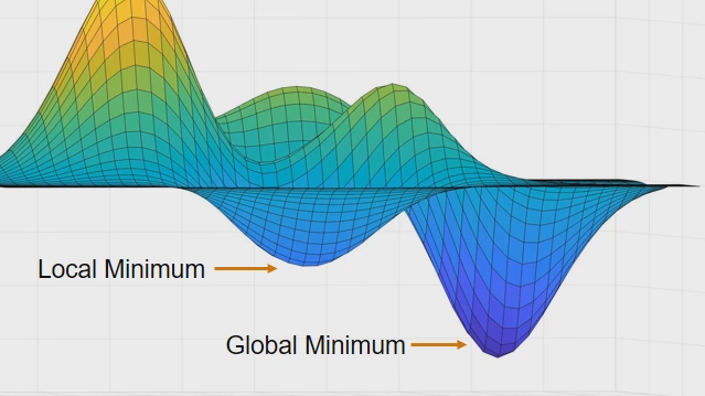
Gradient descent

Outline:

• Start with some \(\theta_0, \theta_1\) (eg. \(\theta_0 = 0, \theta_1 = 0\))
• Keep changing \(\theta_0, \theta_1\) to reduce \(J(\theta_0, \theta_1)\) to find the minimum.

Algorithm

• Repeat until convergence: \(\theta_j = \theta_j - \alpha\frac{\partial }{\partial \theta_j}J(\theta_0,\theta_1)\)

Simultaneous update

• temp_0 \(=\theta_0 - \alpha \frac{\partial}{\partial \theta_0}J(\theta_0, \theta_1)\)
• temp_1 \(=\theta_1 - \alpha \frac{\partial}{\partial \theta_1}J(\theta_0, \theta_1)\)
• \(\theta_0\) = temp_0
• \(\theta_1\) = temp_1

As definition, \(J(\theta_0, \theta_1)\) is a quadratic function.

Derivative of \(J(\theta_0, \theta_1)\)

Here is an example of the derivative through a one variable function. Other multivariate functions are similar.

Step 1: The derivative of the sum is equal to the sum of the derivatives.

Step 2: Apply power rule and Chain rule. We have:

Step 3: Totally, \(\frac{\partial}{\partial\theta_0}J(\theta_0, \theta_1)=\frac{1}{m}\sum_{i=1}^m\:\left(\theta_0+\theta_1x_i-y_i\right)\)

Similar to \(\theta_0\), \(\frac{\partial}{\partial \theta_1}J(\theta_0, \theta_1)=\frac{1}{m}\sum_{i=1}^m\:x_i(\theta_0 + \theta_1x_i-y_i)\)

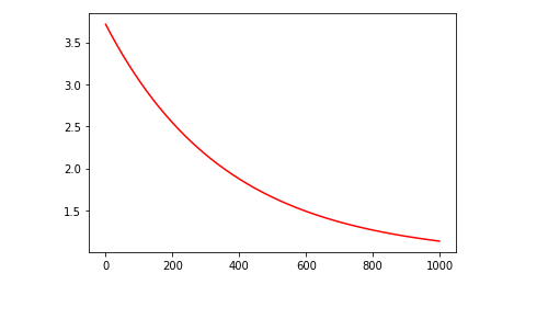
Gradient descent algorithm

Above we have the derivative which is the decrease of the function J. If want to control the reduce of theta, we have the learning rate. Set that to 0.0000001 -> 0.001 would be reasonable for a good accuracy.

Repeat until convergence (with amount iteration) {

• temp_0 \(=\theta_0-\alpha \frac{1}{m}\sum_{i=1}^m\:(\theta_0 + \theta_1x_i-y_i)\)
• temp_1 \(=\theta_1 - \alpha\frac{1}{m}\sum_{i=1}^m\:x_i(\theta_0 + \theta_1x_i-y_i)\)
• \(\theta_0=\) temp_0
• \(\theta_1=\) temp_1 }

Importance

Apply the matrix vectorization to the general case as follows:

Cost function:

Gradient Descent

Source code with python

Analysis and visualize before training

Using seaborn or matplotlib to visualize for an overview of the data set. In seaborn, can use jointplot or pairplot

Data Preprocessing

More details in here

Compute Cost function

# to monitor the convergence by computing the cost.
def computeCost(X, y, theta):
    r = X @ w - y
    return 0.5*np.sum(r*r)

Gradient Descent

def GradientDescentMulti(X, y, theta, alpha):
    m = float(len(y))
    theta = theta - (alpha / m) * (X.T @ (X @ theta - y))
    return theta

Training model

#training(X, y, theta, alpha, iters, cost):
for i in range(0, iters):
    r = X_train @ theta - y_train
    cost[i] = 0.5*np.sum(r*r)
    theta = GradientDescentMulti(X_train, y_train, theta, alpha)

Linear Regression with scikit-learn

from sklearn.linear_model import LinearRegression
from sklearn.model_selection import train_test_split

X = df.iloc[:, :2]
y = df.iloc[:,2]
X_train, X_test, y_train, y_test = train_test_split(X_, y_, test_size=0.3, random_state=42)
lm = LinearRegression()
lm.fit(X_train, y_train)

prediction = lm.predict(X_test)
plt.scatter(y_test, prediction)

This END! Thank for reading !!!

References

1. Machine Learning Andrew Ng
2. More detail of source code: Simple Linear Regression or Multiple Linear Regression